Examples

Numerical experiments from the paper "Computation of optimal transport on discrete metric measure spaces" (Erbar, Rumpf, Schmitzer, Simon).

Each script is self-contained and writes its output (.jld2 data file and/or .pdf figures) to the directory it is run from.

Setup

The examples use a separate Julia environment that includes plotting and data dependencies not required by the package itself. From the repo root:

julia --project=examples

Then instantiate once:

julia> import Pkg; Pkg.instantiate()

After that, run any script with:

julia --project=examples examples/<ScriptName>.jl

Massachusetts experiments additionally require the MA House Districts shapefile from MassGIS. See the header of MassachusettsBarycenter.jl for download instructions.

Experiment descriptions

Synthetic graph experiments

Script	Description
`CubeBarycenter.jl`	Discrete transport barycenter of four measures on the cube graph (8 nodes). Produces a 2×2 reference panel alongside the barycenter.
`HypercubeBarycenter.jl`	Barycenter on the unweighted and randomly weighted 4-dimensional hypercube (16 nodes), visualised with a Schlegel diagram.

ODE validation

Script	Description
`ErbarODE.jl`	Validates the WGD barycenter against an explicit ODE solution on the two-point space. Compares discrete transport, WGD barycenter, and Euler ODE across 1000 time steps; produces six diagnostic figures.

Geodesic and barycenter recovery

Script	Description
`GeodesicRecovery.jl`	Tests coordinate recovery on the triangle graph. Synthesises barycenters along a geodesic, recovers barycentric weights, and measures relative error. Includes a randomised trial producing an error histogram.
`SynthesisAnalysis.jl`	Evaluates synthesis–analysis round-trip accuracy on grid graphs. Computes random barycenters and measures weight-recovery error as a function of iterations.

Grid graph experiments

Script	Description
`GridComparison.jl`	Compares the discrete transport barycenter (joint SOCP) with Sinkhorn barycenters (shortest-path and diffusion-distance costs) on a 7×7 grid, with coordinate recovery for each.
`InitializationsGrid.jl`	Benchmarks sensitivity to warm-start initialisation on a 5×5 grid with five reference measures.
`GridStepSizeVariations.jl`	Sweeps over geodesic step-count parameters on a 4×4 grid, reporting timing and output distance for cold vs. warm starts.

USA state graph experiments

These experiments use the 49-node contiguous-USA graph (one node per state plus DC) constructed from adjacency.

Script	Description
`StatesComparison.jl`	Side-by-side comparison of the discrete transport (SOCP), Sinkhorn/shortest-path, and Sinkhorn/diffusion-distance barycenters on the USA graph.
`EntropicComparison.jl`	Detailed comparison of Sinkhorn barycenters at diffusion-distance costs with varying time parameter `t ∈ {2, 4, 8, 16}` with coordinate recovery by `analysis(method=:sinkhorn)`; California, Maine, and Tennessee as reference measures.
`StateInitializations.jl`	Benchmarks initialisation sensitivity on the USA graph with five geographically concentrated reference measures.
`ParameterVariationsUSA.jl`	Heatmap of coordinate-recovery error across a grid of `(geodesic_steps, geodesic_tol)` parameter values on the USA graph.
`WarmStartBenchmark.jl`	Timing comparison of cold vs. warm-started barycenter computation on the USA graph.
`StateStepVariations.jl`	Investigates synthesis–analysis step consistency: synthesises at `N ∈ {4, 16, 32}` geodesic steps and analyses at all values, producing a 3×3 error matrix.
`BCMDemo.jl`	Visualises the Barycentric Coordinate Manifold on the USA graph: seven barycenters arranged in a triangle according to their recovered weights.

Massachusetts House district graph experiments

These experiments use the 160-node Massachusetts House of Representatives district graph derived from the 2021 MassGIS shapefile (rook adjacency). Run MassachusettsBarycenter.jl first to generate the cached Markov chain.

Script	Description
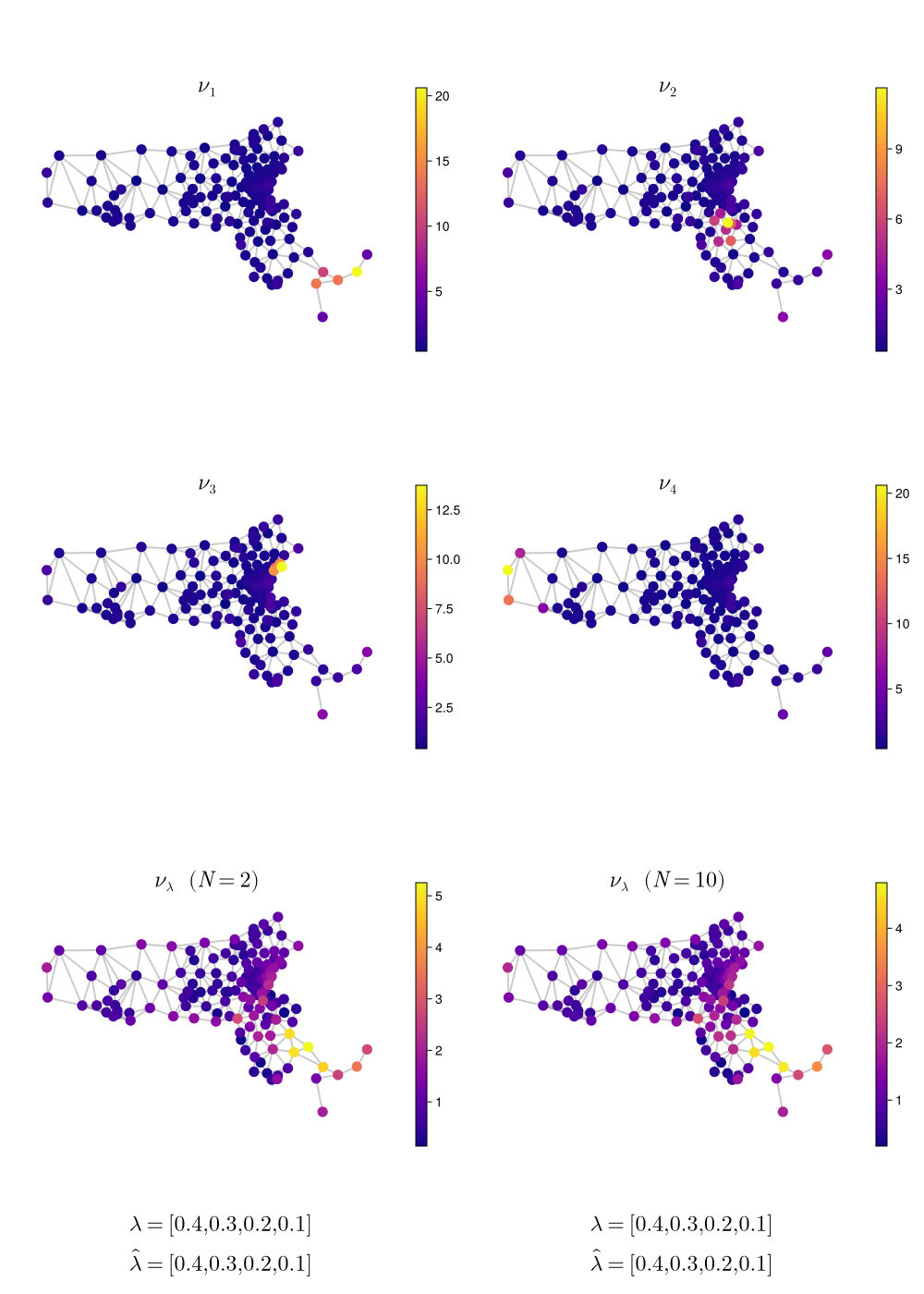
`MassachusettsBarycenter.jl`	Computes the barycenter of four geographically concentrated measures on the MA House graph via the joint SOCP (`barycenter`) at two time resolutions, with coordinate recovery via `analysis`.
`MassachusettsGeodesic.jl`	Visualises the discrete transport geodesic between two geographically distant districts (nodes 5 and 145) in five time frames.

Barycenter of four reference measures on the MA House graph:

MA House barycenter